Research > Metrics > Extratropical Modes of Variability
Extratropical Modes of Variability
RMSE Portrait Plots
(Click thumbnail image for the interactive version for CMIP5 historical)
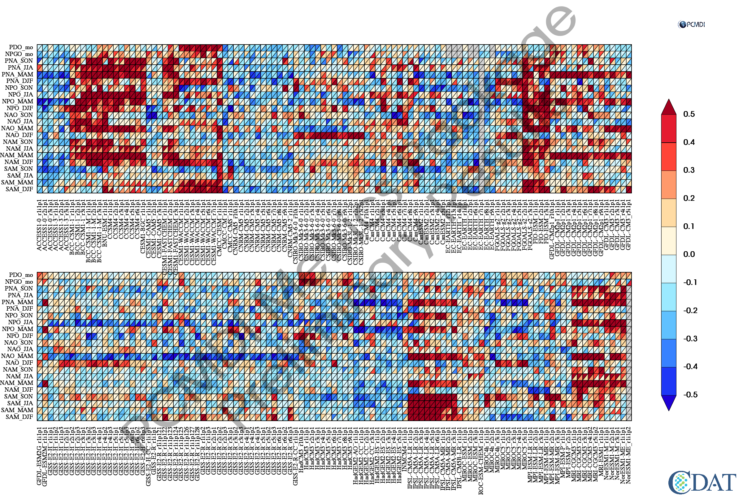
The RMSE Portrait Plots for the modes of variability are akin to Fig. 13a from Lee et al. (2019). For CMIP5 and CMIP6 they show the RMSE relative to the median RMSE of all respective simulations for each mode and season. The RMSE contains errors that arise both in terms of pattern error and amplitude error. The mode/season results for all models are organized by rows, whereas the results from individual realizations across all modes and seasons are isolated by columns. In each cell the normalized results are shown, with for example a result of 0.50 indicating the model RMSE is 50% greater than the median RMSE, whereas a result of −0.25 reflects an error that is 25% smaller than the median of all model results for that particular mode and season. Finally, the upper-left triangle in each cell depicts results based on our default reference (20CR for the sea-level pressure based modes, HadISSTv1.1 for the PDO and NPGO), whereas the results in the lower-right triangle are based on our first alternate source (ERA-20C for sea-level pressure based modes, HadISSTv2.1 for the PDO).
For the RMSE, the advantage of the Portrait Plot is that:
- It allows us to show on a single plot the model performance irrespective of the units of the variable under consideration and/or where the range of the absolute RMSE is different between modes/seasons
- It preserves the relative model performance with respect to the observations
- It gives an indication of how well a given model is performing in a multi-model context
The Portrait Plots are interactive. Clicking on any cell triangle will give its associated value, the observed EOF’s using our primary and secondary observed datasets, EOF’s 1-3 of the model, the model CBF EOF, and the PC time series of the EOF’s and the CBF EOF. Clicking on a mode along the y-axis will give the associated Taylor Plot of all models for that mode/season.
Summary statistics in RMSE Portrait Plots
General Conclusions
There are several general conclusions that we can draw from the RMSE Portrait Plots. Firstly, though the selection of a reference dataset is important, it does not radically impact the general conclusions about a particular model’s agreement with the observed EOF spatial pattern. Secondly, with some binning of the results (the color bar uses 10% increments), we see that in many cases the results for a given model’s relative performance is not very sensitive to which realization is examined. Our results are thus fairly robust to internal variability and selection of reference data. A more detailed discussion of the RMSE results are given in Lee et al. (2019).
—
Amplitude Portrait Plots
(Click thumbnail image for the interactive version for CMIP5 historical)
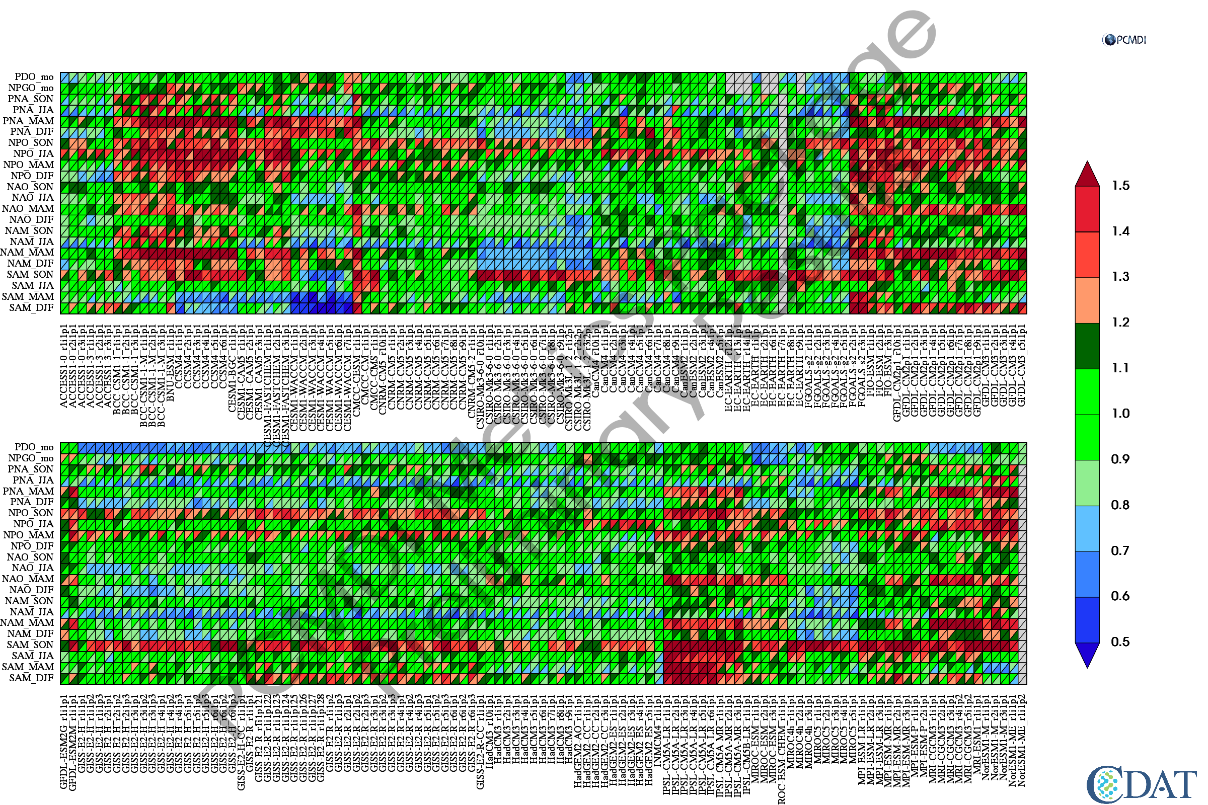
The amplitude Portrait Plots for the modes of variability are akin to Fig. 14 from Lee et al. (2019). It gives the standard deviation of the model CBF PC time series divided by the standard deviation of the observed PC time series such that values close to one indicate consistency between the models and observations.
The Portrait Plots are interactive. Clicking on any cell triangle will give its associated value, the observed EOF’s using our primary and secondary observed datasets, EOF’s 1-3 of the model, the model CBF EOF, and the PC time series of the EOF’s and the CBF EOF. Clicking on a mode along the y-axis will give the associated Taylor Plot of all models for that mode/season.
Summary statistics in Amplitude Portrait Plots
General Conclusions
It is notable that for the majority of amplitude cells the model-to-observed reference ratios are within 0.9–1.1. There is substantial overlap between the RMSE Portrait Plots and the amplitude Portrait Plots. In particular, the amplitude outliers reinforce other Lee et al. (2019) evidence that temporal amplitude errors dominate the RMSE in many cases. Additionally, the results indicate a systematic error in the season immediately following the dominant season during which nearly 80% or more of the models overestimate the temporal variability. The post-dominant season overestimate suggests that the dominant season (winter) mode is too persistent compared to observations, though this hypothesis requires further investigation.
Reference
Lee, J., Sperber, K.R., Gleckler, P.J., Bonfils, C.J. and Taylor, K.E., 2019. Quantifying the agreement between observed and simulated extratropical modes of interannual variability. Climate Dynamics, 52: 4057-4089, doi: 10.1007/s00382-018-4355-4.

